Documentation
Cell Type Proportion Analysis
Introduction
This function allows users to keep samples in the sub-datasets (tissues from GTEx or cancer types from TCGA) they selected, and filter the cell types of interest to visualize and compare their proportions in each bulk sample. Up to five sub-datasets are supported.
After clicking the "plot" button, the interactive boxplots grouped by cell type and sub-dataset will be available. The one-way ANOVA function has been dynamically integrated into each sub-group in each boxplot, allowing users to have a quantitative comparison of the cell proportions.
Parameters
- TCGA Tumor/TCGA Normal/GTEx/Used Expression Datasets: Select cancer types of interest in the "TCGA Tumor", "TCGA Normal" or "GTEx" field and click "add" to build dataset list in the "Used Expression Datasets" field. Also, manual input of cancer types split by comma (e.g. COAD Tumor,READ Tumor) is also acceptable. The cell type proportion analysis is based on the datasets list.
- Cell Types: Select cell types of interest for analysis.
- Normalization: For each sample, normalize the proportions of selected cell types to make the sum equal to 1.
Results
Click the “Plot” button: GEPIA will generate interactive box plots based on input parameters with two different grouping methods.
Grouped by tissue
For samples in each sub-dataset (e.g. LIHC Tumor), this plot allows users to quantitatively compare the proportion distributions of different cell types.
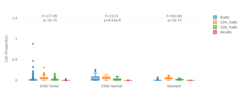
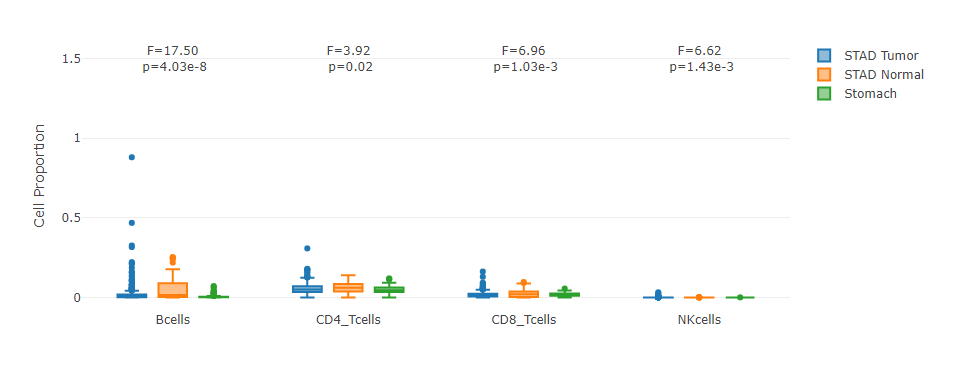
Grouped by cell type
For each cell type, this plot allows users to quantitatively compare its proportion distribution across samples in different sub-datasets.
Cell Type Correlation Analysis
Introduction
This function allows users to keep samples in the sub-datasets (tissues from GTEx or cancer types from TCGA) they selected, and select two cell types of interest to perform the correlation analysis across bulk samples. Up to five sub-datasets are supported.
After clicking the "plot" button, the interactive scatter plot colored by sub-dataset will be available. The Pearson Correlation Coefficient will be dynamically calculated, allowing users to have a quantitative metric for the proportion correlation between the two cell types selected.
Parameters
- TCGA Tumor/TCGA Normal/GTEx/Used Expression Datasets: Select cancer types of interest in the "TCGA Tumor", "TCGA Normal" or "GTEx" field and click "add" to build dataset list in the "Used Expression Datasets" field. Also, manual input of cancer types split by comma (e.g. COAD Tumor,READ Tumor) is also acceptable. The cell type proportion analysis is based on the datasets list.
- Select cell types for comparison: : Select two cell types of interest for the correlation analysis.
Results
Click the “Plot” button: GEPIA will generate interactive scatter plot based on input parameters.
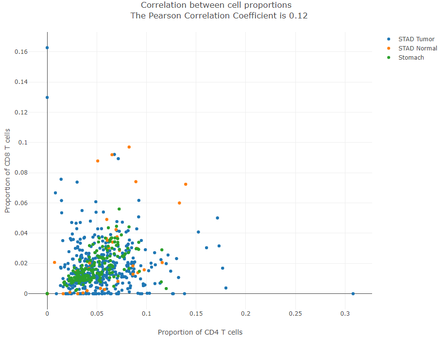
Correlation scatter plot
For samples in sub-datasets selected, this plot allows users to quantitatively analyze the correlation between the proportions of two cell types. The data points (samples) are colored by sub-dataset.
Cell Type-level Expression Analysis
Introduction
This function allows users to keep samples in the sub-datasets (tissues from GTEx or cancer types from TCGA) they selected, and enables users to perform the differential expression in the cell type-level. Up to five sub-datasets are supported.
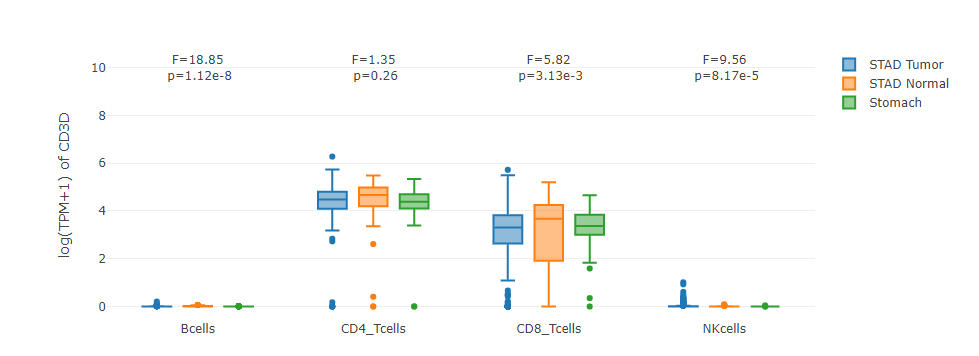
After clicking the "plot" button, the interactive boxplots grouped by cell type and sub-dataset will be available. The one-way ANOVA function has been dynamically integrated into each sub-group in each boxplot, allowing users to simutenously visualize and compare the gene expression in given cell types.
Parameters
- TCGA Tumor/TCGA Normal/GTEx/Used Expression Datasets: Select cancer types of interest in the "TCGA Tumor", "TCGA Normal" or "GTEx" field and click "add" to build dataset list in the "Used Expression Datasets" field. Also, manual input of cancer types split by comma (e.g. COAD Tumor,READ Tumor) is also acceptable. The differential expression analysis is based on the datasets list.
- Cell Types: Select cell types of interest for analysis.
- Input Gene(s): Input the gene symbol for analysis. You can input the gene in GEPIA in order to verify the correctness of the gene symbol or convert the gene ID or gene alias into the standard gene symbol.
Results
Click the “Plot” button: GEPIA will generate interactive box plots based on input parameters with two different grouping methods.
Grouped by tissue
For samples in each sub-dataset (e.g. LIHC Tumor), this plot allows users to quantitatively compare the gene expression distributions contributed by different cell types.
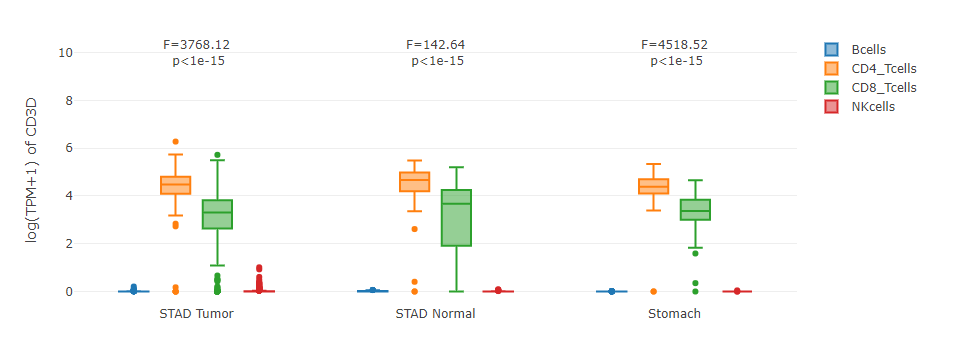
Grouped by cell type
For each cell type, this plot allows users to quantitatively compare the gene expression distribution across samples in different sub-datasets.
Cell Type-level Survival Analysis
Introduction
Users can first choose the range of sub-datasets, and then separate the samples into two groups, according to the total proportion of cell cell types selected. In addition, we also apply the log-rank test to check whether the two K-M curves are statistically different. The p-value of the log-rank test will be displayed in the title of the survival plot. Up to five sub-datasets are supported.
Parameters
- TCGA Tumor/Used Datasets: Select cancer types of interest in the "TCGA Tumor" and click "add" to build dataset list in the "Used Expression Datasets" field. Also, manual input of cancer types split by comma (e.g. COAD Tumor,READ Tumor) is also acceptable. The correlation analysis is based on the datasets list.
- Cell types: Select cell type(s) of interest for analysis. If more than one cell types are selected, we will use the sum proportion of them.
- Cutoff-high: Samples with the sum proportion of selected cell type(s) higher than this threshold are considered as the high-expression cohort (red lines in the survival plot).
- Cutoff-low: Samples with the sum proportion of selected cell type(s) lower than this threshold are considered as the low-expression cohort (blue lines in the survival plot).
- Type of survival periods: Select "Overall Survival" or "Relapse-free Survival" data of TCGA tumor samples for analysis.
- Show 95% confidence interval: Select whether to show the 95% confidence interval of each K-M curve.
- Show right censoring mark: Select whether to show the + mark on the K-M curve for each right-censored sample.
Results
Click the “Plot” button: GEPIA will generate interactive Kaplan-Meier survival plots based on input parameters.
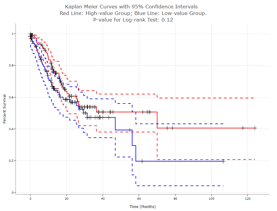
Kaplan-Meier plots
This plot allows users to quantitatively visualize and compare the survival curves of two sample groups. For example, here we first filter samples from the LIHC sub-dataset, rank the samples according to the B cell proportion, and assign the top 30% and bottom 30% samples as the "high-group" and "low-group" (by setting "Cutoff-high %" to 70 and "Cutoff-low %" to 30), respectively. For any time point, users can hover the plots to see the exact survival percentage, its 95% confidence intervals, or the right censored observations. The smaller the p-value is, the more statistically different the two K-M curves will be.
TCGA/GTEx Data Information
We downloaded the TCGA (version 2016-09-01) and the GTEx (version 2016-04-19) expression data from the UCSC XENA Data Hubs.
Transcripts Per Million (TPM) matrices of the two datasets were re-calculated on the approved protein-coding genes.
Here is the information table on the abbreviation of TCGA cancer types, the sample numbers of each datasets and the tumor-normal pairs of TCGA/GTEx sub-datasets as proposed in GEPIA1/2.
| TCGA | Detail | Tumor | Normal | GTEx | Num |
| ACC | Adrenocortical cancer | 77 | - | Adrenal Gland | 128 |
| BLCA | Bladder Urothelial Carcinoma | 407 | 19 | Bladder | 9 |
| BRCA | Breast invasive carcinoma | 1099 | 113 | Breast | 179 |
| CESC | Cervical squamous cell carcinoma and endocervical adenocarcinoma | 306 | 3 | Cervix Uteri | 10 |
| CHOL | Cholangio carcinoma | 36 | 9 | - | - |
| COAD | Colon adenocarcinoma | 290 | 41 | Colon | 308 |
| DLBC | Lymphoid Neoplasm Diffuse Large B-cell Lymphoma | 47 | - | Blood | 444 |
| ESCA | Esophageal carcinoma | 182 | 13 | Esophagus | 653 |
| GBM | Glioblastoma multiforme | 166 | 5 | Brain | 1152 |
| HNSC | Head and Neck squamous cell carcinoma | 520 | 44 | - | - |
| KICH | Kidney Chromophobe | 66 | 25 | Kidney | 28 |
| KIRC | Kidney renal clear cell carcinoma | 531 | 72 | Kidney | 28 |
| KIRP | Kidney renal papillary cell carcinoma | 289 | 32 | Kidney | 28 |
| LAML | Acute Myeloid Leukemia | 173 | - | Bone Marrow | 70 |
| LGG | Brain Lower Grade Glioma | 523 | - | Brain | 1152 |
| LIHC | Liver hepatocellular carcinoma | 371 | 50 | Liver | 110 |
| LUAD | Lung adenocarcinoma | 515 | 59 | Lung | 288 |
| LUSC | Lung squamous cell carcinoma | 498 | 50 | Lung | 288 |
| MESO | Mesothelioma | 87 | - | - | - |
| OV | Ovarian serous cystadenocarcinoma | 427 | - | Ovary | 88 |
| PAAD | Pancreatic adenocarcinoma | 179 | 4 | Pancreas | 167 |
| PCPG | Pheochromocytoma and Paraganglioma | 182 | 3 | - | - |
| PRAD | Prostate adenocarcinoma | 496 | 52 | Prostate | 100 |
| READ | Rectum adenocarcinoma | 93 | 10 | Colon | 308 |
| SARC | Sarcoma | 262 | 2 | - | - |
| SKCM | Skin Cutaneous Melanoma | 469 | 1 | Skin | 812 |
| STAD | Stomach adenocarcinoma | 414 | 36 | Stomach | 174 |
| TGCT | Testicular Germ Cell Tumors | 154 | - | Testis | 165 |
| THCA | Thyroid carcinoma | 512 | 59 | Thyroid | 279 |
| THYM | Thymoma | 119 | 2 | Blood | 444 |
| UCEC | Uterine Corpus Endometrial Carcinoma | 181 | 23 | Uterus | 78 |
| UCS | Uterine Carcinosarcoma | 57 | - | Uterus | 78 |
| UVM | Uveal Melanoma | 79 | - | - | - |
| Adipose Tissue | 515 | ||||
| Blood Vessel | 606 | ||||
| Fallopian Tube | 5 | ||||
| Heart | 377 | ||||
| Muscle | 396 | ||||
| Nerve | 278 | ||||
| Pituitary | 107 | ||||
| Salivary Gland | 55 | ||||
| Small Intestine | 92 | ||||
| Spleen | 100 | ||||
| Vagina | 85 |
Frequently Asked Questions
Q1:What is the motivation to develop GEPIA2021?
A1:We launched GEPIA project in 2017 to facilitate the widely used analysis on the expression datasets TCGA and GTEx, providing the biologists and clinicians with a handy tool to perform comprehensive and complex data mining tasks. Until the end of 2020, GEPIA and GEPIA2 have been totally cited for ~2,600 times, and have processed ~1,300,000 analysis requests for ~300,000 users worldwide. Based on the feedbacks, we decided to develop GEPIA2021, an extended version of GEPIA with multiple cell type-level analysis based on bulk sample deconvolution results.
Q2:How to select the deconvolution tool among CIBERSORT, EPIC and quanTIseq?
A2: CIBERSORT is recommended when users want to investigate the immune cell types with high resolution (providing cell sub-types such as T.cells.CD4.memory.activated). EPIC provides the reference with two non-immune cell types but the least immune cell types. The strategies to estimate the absolute proportion of all three tools are basically similar,and thus, the cell proportions of different samples become comparable. For example, CIBERSORT estimates the proportion of each cell type against the total immune cell content first, and then estimates the immune cell content in the mixture by the median gene expression of the s signature genes (in formula ii) against the median of all genes, based on the assumption that the signature gene expression cannot be contributed by other cell types beyond the reference. Notably, the absolute proportion output is natively supported by EPIC and quanTIseq, while the absolute_mode in CIBERSORT is still a beta version. The numbers of genes available for sub-expression analysis differ in three tools, which depend on the references provided by the tools. According to the publications of the 3 tools, CIBERSORT was designed for multiple type of tissues, while EPIC and quanTIseq were orginally designed for tumor samples. Therefore, we would recommend CIBERSORT as the first choice for the tumor-normal comparison. However, as all three tools were extensively validated on normal blood and tumor samples, there is still potential applicability for the usage of EPIC/quanTIseq on the blood cell deconvolution on GTEx samples. In addition, EPIC/quanTIseq also achieved high performance in this benchmark article.
Q3:Why do you build a standalone extension rather than integrating the functionalities into the origin version of GEPIA?
A3:Please let us first introduce our data processing workflow. We downloaded TCGA and GTEx data from Xena. We only keep the intersection set of genes between the downloaded data and the reference, and perform the log-normalization and downstream analysis based on these genes. Therefore, the expression of genes used for GEPIA2021 would be different from that of GEPIA/GEPIA2.
Q4:How do you explain the ANOVA results in the Proportion and the Sub-expression modules?
A4:By assuming that there is no difference in variance among all groups, we perform the F-test (one-way ANOVA) to identify the degree of difference, along with the p-value indicating the significance. If the p-value is too small (1e-16, comparable with the floating-point precision), it will be shown as zero. If the compared groups have all samples with zero proportion or expression, the F-value and p-value will be NAN.
Code Availability
The codes for the bulk data deconvolution can be accessed here.